
Parsing NASA thermodynamic data using MATLAB
AIM:
The aim of this project is to write a MATLAB program that can read a file that contains thermodynamic data in a polynomial format (eg. files from CHEMKIN II).
OBJECTIVES OF THE PROJECT:
The above file contains a set of compounds for which a set of coefficients are given. These coefficients are used in the above equation to get the values for Cp, enthalpy, and entropy. Each compound or gas contains 14 coefficient and the first 7 coefficients are to be used if the temperature are high and the next 7 coefficients are to be used if the temperatures are low.
Also, the high, low mid temperatures for each compound are mentioned. Using this data, the coefficients and the thermodynamic values are to be extracted. The molecular mass of a particular species is also to be calculated. After getting the required thermodynamic values each individual value is to be plotted against the local temperature These files are to be saved as images with appropriate names and these images are to be stored in a folder specific to a particular species.
PROCEDURE:
Parsing is the process of splitting data into chunks of information that are easier to manipulate and store. We parse the thermodynamic data to extract useful information from it. To do that I’ve followed this procedure.
The given file is taken as an input and fed into a string array line by line. The first line is the heading so no changes required with that. The second line is the global temperature values so I extracted the temperatures from the second line by splitting them exactly at the spaces used between the words These string temperature values are then converted into numerical values. The next three lines are comments passed by NASA to deal with the data file so no changes required with that and we store it as it is. Now if we observe the lines from 6 to the end are in a particular format. The first line in this format would include the species name, species ID, No of atoms in a particular species, Physical state, Local temperature values, and the row number The remaining three lines of this format would simply have the coefficients. So, I wrote a set of instructions to extract the species names, their temperatures, and their coefficients that start from the 6th line, skip 3 lines and then 10th, and so on to 214th The instructions were given in such a way that the program would know that the 6th line starting term is the species name and the last but one temperature is the mid local temperature, the second last is the highest local temperature and the third last temperature is low local temperature. The extracted temperatures were fed into another temperature array. The species ID and atoms in the gases were inseparable and the procedure would become more complex if we try to extract them and since our focus was on extracting coefficients, we move on to the next line So, the program would identify the coefficients by identifying the positions of E in the lines The terms till E and the next three terms from E together are considered to be one coefficient, the same is applied for all the lines. Now since we got the temperatures and the coefficients, we move on to calculating the thermodynamics For our ease of understanding the program, a separate function is written to find out these thermodynamic values. This program is based on the formula above the temperature values are simply plugged into the formula to get the values. Also, another condition is implemented in the function that for a range of temperatures ranging from mid local temperature to high local temperature the first 7 coefficients are to be used, and for temperatures ranging from low local temperature to mid local temperature, the second 7 coefficients are to be used. This forms an array of values for the three thermodynamic parameters. The array depends on the range of temperature provided. Another function is written to calculate the molecular mass of species. This function takes the species name, compares it with the data set provided, and if the name matches then the program will add the mass. It also takes the polyatomic gases into consideration and adds the mass accordingly. The generated mass for each species is then displayed in the command window using a printf command. Now for the program to generate plots and store them in a separate folder, we need to create a folder first and change the MATLAB operating directory into that folder and then store the plots and come back to the original directory where all the programs are stored. This procedure can be used for all species. The code employs the same. To save the plots we use a command called save as where it saves the file into the format specified in the current operating directory. The format used here is JPG format. After the file saving is complete the current directory is changed back to the program directory and the end of the loop.
If everything is in place the program should look like this
clear all
close all
clc
%opening the thermo.dat with read only permissions
f1 = fopen('THERMO.dat','r');
%reading the file line by line
tline = fgetl(f1);
i = 1;
L = string(100);
while ischar(tline)
L(i) = tline;
i=i+1;
tline = fgetl(f1);
end
%Header
disp(L(1));
%2nd line global temperature values
L_2_split = strsplit(L(2),' ');
%splitting the second line using the delimiter
%converting them to number
g_l_t = str2double(L_2_split{2});
g_m_t = str2double(L_2_split{3});
g_h_t = str2double(L_2_split{4});
disp('global temperature values')
fprintf('Low temp:%dn',g_l_t)
fprintf('Mid temp: %dn',g_m_t)
fprintf('High temP: %dn',g_h_t);
%3,4,5 lines are comments so I leave them be.
disp(L(3));
disp(L(4));
disp(L(5));
%Parsing the species block
for j = 6:4:214
%Starting fro 6th line is the name of the species and the same repeats
%after every 4 lines so the above logic is used to identify the species
%name
spe_head = strsplit(L(j),' ');
%identifying different parameters by splitting them using the strsplit
%command
q = numel(spe_head);
%identifying no of useful terms in the first line
species_name = char(spe_head(1));
%making sure that the species name is a string
%the species ID and the atoms were inseperable so i clubbed them to from a
%new term and the G represents the physical state of the species at NTP so
%gathered it along with the row number
for h = 2:q-5
id_atoms = spe_head(h)+spe_head(h+1);
physical_state = spe_head(q-4);
spe_row_number = spe_head(q);
end
%starting from right towards left we have the row number and the
%temperatures so i came from right to left to get the local temp values for
%that particular species
l_l_t = str2double(spe_head{q-3});
l_h_t = str2double(spe_head{q-2});
l_m_t = str2double(spe_head{q-1});
%An array of local temp values is constructed
temp = [l_l_t,l_h_t,l_m_t];
%to extract the coefficients i used the following procedure. So the
%coefficients are there in the next line to the line containing the
%species name so i added +1 to go to the next line
f_e = strfind(L(j+1),'E');
%i identified the terms by seperating them at E
a = char(L(j+1));
%i made sure the entire line is in string format
%since the e power has three digits in it i added 3 strings next of e to
%the terms and gathered them
a_num1 = a(1:15);
a_num2 = a(16:30);
a_num3 = a(31:45);
a_num4 = a(46:60);
a_num5 = a(61:75);
%Converting the string terms into numbers using the str2double command
a1 = str2double(a_num1);
a2 = str2double(a_num2);
a3 = str2double(a_num3);
a4 = str2double(a_num4);
a5 = str2double(a_num5);
%the same process is done for other two lines as well
%NOTE the below steps can be reduced by writing another for loop but to
%reduce the complexity i kept the procedure this way
f_e1 = strfind(L(j+2),'E');
b = char(L(j+2));
a_num6 = b(1:15);
a_num7 = b(16:30);
b_num1 = b(31:45);
b_num2 = b(46:60);
b_num3 = b(61:75);
a6 = str2double(a_num6);
a7 = str2double(a_num7);
b1 = str2double(b_num1);
b2 = str2double(b_num2);
b3 = str2double(b_num3);
f_e2 = strfind(L(j+3),'E');
c = char(L(j+3));
b_num4 = c(1:15);
b_num5 = c(16:30);
b_num6 = c(31:45);
b_num7 = c(46:60);
b4 = str2double(b_num4);
b5 = str2double(b_num5);
b6 = str2double(b_num6);
b7 = str2double(b_num7);
%Generating a range of local temperature values
T = linspace(temp(1),temp(2),100);
%Generating an array of the coefficients These arrays are generated for the
%ease of feeding them into subfunctions
coeff = [a1,a2,a3,a4,a5,a6,a7,b1,b2,b3,b4,b5,b6,b7];
M = molecular_weight(species_name);
%printing the molecular mass of obtained from the molecular_weight function
%It is actually supposed to be mass not weight
fprintf('molecular mass of %s is %fn',species_name,M)
%thermo_prop function to obtain the values of enthalpy,entropy and specific
%heat constant
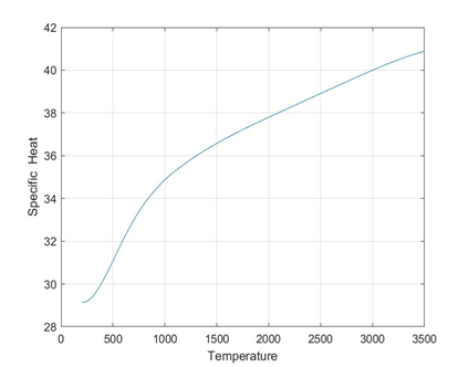
%Notice the specific heat tends to increase as the temperature increases
[Cp,H,S] = thermo_prop(temp,coeff);
%creating a directory
mkdir(species_name)
%changing the current PWD to the created file
cd(species_name)
%plotting
f = figure('name',species_name);
plot(T,Cp)
xlabel('Temperature')
ylabel('Specific Heat')
grid on
%saving using the saveas command the format to be saved is specified as jpg
saveas(f,species_name,'jpg')
%closing the graphs would be a better option compared to our PC getting
%fried up
close(f)
%same set of commands are used for the next two graphs as well
%NOTE the below graphs can also be looped into a for loop but for the sake
%of experimentation using different commands i chose to keep them seperate
g = figure('name',species_name);
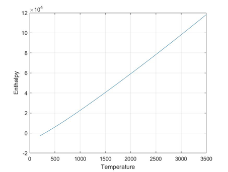
plot(T,H)
xlabel('Temperature')
ylabel('Enthalpy')
grid on
name = strcat(species_name,'H');
saveas(g,name,'jpg')
close(g)
y = figure('name',species_name);
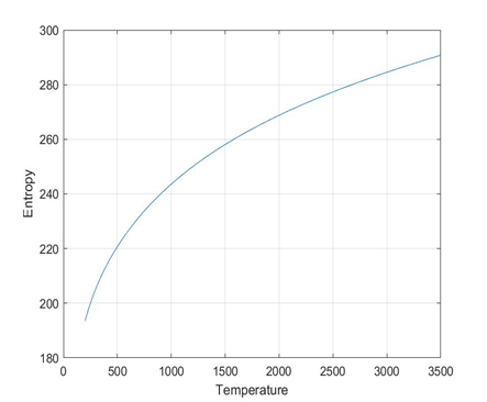
plot(T,S)
xlabel('Temperature')
ylabel('Entropy')
grid on
filename = strcat(species_name,'S');
saveas(y,filename,'jpg')
close(y)
%getting back into our original directory. This is important as the
%directory of matlab changes we have to change it back to where the
%programs are going to be saved.
cd ..
end
%Footer
disp(L(218));
The program for molecular mass function
function M = molecular_weight(species_name)

%The given NASA file elements have been taken into consideration if the
%NASA file has more elements they can be added using loops
element = ['H','C','O','N','A','S'];
%NOTE that the notation for argon gas has been given as A instead of AR
%this is because matlab takes a, r as two seperate inputs instead of one so
%if we have to know the properties of argon gas the input must be A

%The atomic weight of the above elements are fed into an array
%NOTE the atomic weights are added in the same order as above
atomic_weight = [1.0079 12.0107 15.999 14.0067 39.948 32.065];

atom_num = ['2','3','4','5','6','7','8','9','10'];
%the no of atoms in the compound is fed this can also be done in a more
%efficeint way

%STRCMP string compare command is used for comparing the user input and the
%data base i.e the element array
M = 0;
for n = 1:length(species_name)
    for u = 1:length(element)
        if strcmp(species_name(n),element(u))
           %the above command compares the strings of the mentioned and if
           %they match then the below step is executed if not the below
           %loop is executed
            M = M + atomic_weight(u);

        else
            for v= 1:length(atom_num)
                if strcmp(species_name(n),atom_num(v)) &&  n>1 && strcmp(species_name(n-1),element(u))
                    %The above 3 conditions are required to identify
                    %polyatomic gases

                    k = str2double(atom_num(v));
                    M = M + ((atomic_weight(u))*(k-1));
                end
            end
        end
    end
end
end
The program for thermodynamic properties function
function [Cp,H,S] = thermo_prop(temp,coeff)
%Defining universal gas constant
R = 8.315; %unit: m2 kg s-2 K-1 mol-1
%creating a temperature range
T = linspace(temp(1),temp(2),100);
%for both low temperature and high temperature the Cp values are taken and
%are plugged in to obtain specific heat , entropy and enthalpy at different temperatures.
for i = 1:length(T)
if T(i)>= temp(3)
    %since the first 7 coefficients are High temperature coefficients
    a = coeff(1:7);
    %For our conveinience we manipulated the given formula such that LHS
    %contains only the values required.
    Cp(i) = (a(1)*R) + (a(2)*T(i)*R) + (a(3)*(T(i)^2)*R) + (a(4)*(T(i)^3)*R) + (a(5)*(T(i)^4)*R);
    H(i)= (a(1)*R*T(i)) + (a(2)*(T(i)^2)*R/2) + (a(3)*(T(i)^3)*R/3) + (a(4)*(T(i)^4)*R/4) + (a(5)*(T(i)^5)*R/5) + (a(6)*R);
    S(i) = (a(1)*R*(log(T(i))) + (a(2)*T(i)*R) + (a(3)*(T(i)^2)*R/2) + (a(4)*(T(i)^3)*R/3) + (a(5)*(T(i)^4)*R/4)+ (a(7)*R));
else
if T(i) < temp(3)
    a = coeff(8:14);
    %The next seven coefficients are for low temperature
    Cp(i) = (a(1)*R) + (a(2)*T(i)*R) + (a(3)*(T(i)^2)*R) + (a(4)*(T(i)^3)*R) + (a(5)*(T(i)^4)*R);
    H(i) = (a(1)*R*T(i)) + (a(2)*(T(i)^2)*R/2) + (a(3)*(T(i)^3)*R/3) + (a(4)*(T(i)^4)*R/4) + (a(5)*(T(i)^5)*R/5) + (a(6)*R);
    S(i) = (a(1)*R*log(T(i))) + (a(2)*T(i)*R) + (a(3)*(T(i)^2)*R/2) + (a(4)*(T(i)^3)*R/3) + (a(5)*(T(i)^4)*R/4)+ (a(7)*R);

end
end

end
RESULTS:
The plots for different species will be generated
plots for O2 species
folders will be created for each species

Each folder will have 3 images 1) plot of cpVst 2)plot of sVst 3) plot of hVst


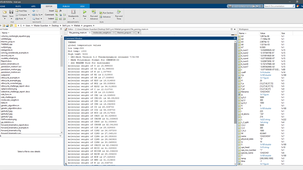
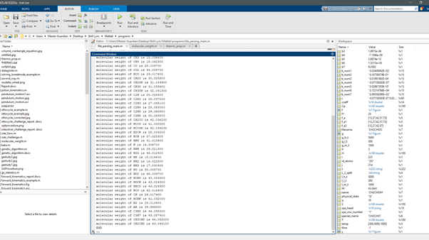
The command window showing the molecular mass of each species
CONCLUSION:
The graphs for different thermodynamic properties are plotted and are saved in different directories automatically. During the programming, the for loops might encounter indexing problems if the variables used are taken care of This project doesn’t store the values of 14 coefficients of all the species it only stores them until the loop is completed and then new 14 values of the next species are stored. This can be improved if the storage is necessary Some of the activities can be simplified more by looping them this might increase the complexity of the code while reducing the length of the code. But for the sake of simplicity, those activities were written in the lengthy method.
REFERENCES:
Format data into string or character vector - MATLAB sprintf - MathWorks India
How can I save multiple plots in a specified folder? - MATLAB Answers - MATLAB Central
Make new folder - MATLAB mkdir
saving an image in a specific folder - MATLAB Answers - MATLAB Central