Flow over ahmed body

AIM:

This project aims to simulate the flow over Ahmed body in Ansys Fluent.

OBJECTIVES OF THE PROJECT:

*Generate Velocity and pressure contours.

*Calculate the drag coefficient plot for a refined case.

*Generate the vector plot clearly showing the wake region.  

*Perform the grid independency test and evaluate the values of drag and lift with each case.  

THEORY

What is an Ahmed body?

The Ahmed body is a geometric shape first proposed by S. R. Ahmed and Ramm in 1984. The shape provides a model to study geometric effects on the wakes of ground vehicles. It can be used to validate CFD solvers. The results of airflow over this body were captured using the wind tunnel experiments and the CFD solver results are compared with these experimental results to find out the accuracy of the solver.

Picture credits : Flow and Turbulence Structures in the Wake of a Simplified Car Model

The above picture represents the ahmed body dimensions. Its virtual version can be found here

PROCEDURE:

Importing the CAD model

The geometry can be created using any standard CAD package. In this case the geometry is already created.

We import the STEP file into Ansys Spaceclaim. Once the geometry appears, we check the geometry units, If the dimensions are in mm. We quickly change the dimensions using File> Spaceclaim Options > Units. And convert them to meters.

To observe the flow over an Ahmed body we create a virtual wind tunnel. This can be created by using the enclosure tool.

But before we create the wind tunnel, we need to know the dimensions of the wind tunnel.

The distance after the Ahmed body should be 5 - 10 times the characteristic length but 10 times the characteristic length requires more computational time and power hence we reduce it to 5 times to accurately capture the wake produced. We also consider only one half of the ahmed body (cut along the length) to go easy on the number of cells required to mesh.

In the z-direction, the total length should be at least 5 times but due to computational restraint we reduce it to 0.5 m

we keep the same length for y as well, Y direction length (from above the Ahmed body) is 1 m

Now we use the enclosure option to create an enclosure on the ahmed body. We then uncheck the original imported geometry, suppress it for physics. This needs to be done to prevent overlapping of bodies.

Now we create another box around the ahmed body, This box will be used for mesh refinement. We use the interference tool to remove the mesh interference. Once this is done we exit the Spaceclaim. This model will be updated to Ansys workbench.

Once created the geometry should like this

Meshing

Now we open the Ansys mesher. Here we first start by naming the boundaries as.

The second box created is for refining the mesh hence we select the mutizone mesh. If we inspect the geometry we can see that the legs of the ahmed body lost their cylindrical shape. This is due to coarse size of the mesh. To regain the shape we use face sizing at the legs. In order to give the refinement we use the edge sizing option to refine the mesh inside the refinement zone. To capture the effects at the car wall we give inflation layers at the car wall. Upon meshing the geometry will look like this.

Case setup

For this project we use a steady state solver. And we use a pressure based solver. This is an external flow hence we use a K Omega SST model to solve for turbulence. The fluid is taken as air and the properties are default. The boundaries are set as follows.

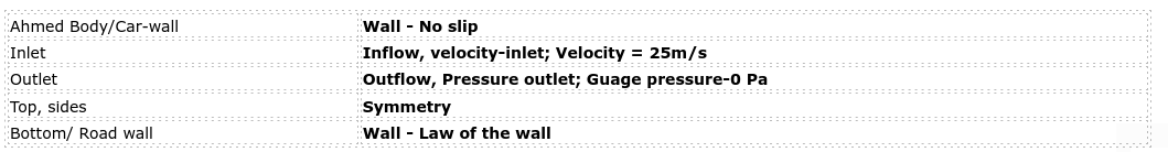
Before we proceed to initialisation we need to take care of the reference values. This is important and incorrect reference values will lead to improper drag and lift values.

Once these values are set we can proceed to initialisation (Hybrid/Standard). Once initialisation is done we get initial velocity contours. We create a plane and observe the velocity contour on that plane. Also we save this animation for future references.

We now run the simulation for 350 iterations and the end results are as follows

Velocity contour

Residual plots

Cd plot

Cl plot

POST PROCESSING:

We can post process the above results to get some important results such as line probes, graphs and vector plots. These are important to identify the point of seperation, recirculation zone etc.

The above vectors are plotted on a plane XY at Z = 163.5 mm.

Recirculation Zone

When an object moves on a fluid, the first layer of the fluid sticks on the surface of the body. When there is a sharp change in the geometry, there comes a point on the body where the fluid detaches from the surface, thus breaking the boundary layer, this point at which the fluid detaches from the surface is called the point of separation. Due to this flow seperation happens and a low pressure zone is created at the end of the ahmed body.This low pressure is again occupied by air from the high pressure. This process is called as recirculation of air and this zone is called as ReCircualtion Zone If we are to take a look at the pressure contour it would look like this. 

Negative Pressure ?

In the above contour, the range of pressure is adjusted so that the negative pressure range can be clearly seen. The explanation as to why there is a negative pressure in the domain goes as follows:

The front of the ahmed body is blunt hence When the air hits the front of the body the air gets stagnated due to which the pressure rises, This can be observed at the front portion of ahmedbody. The area in red indicates the increased pressure. This air eventually passes over the geometry and when ever there is a sharp change in geometry this air tends to expand increasing velocity and losing pressure. This pressure drop causes the negative pressure zones.

Grid Dependency Test

The above case we looked at is the most refined case. We change the mesh size and see if it affects the solution. In the earlier case the size of the grid in the refinement zone is 0.02m. We change the size of the refinement zone to 0.03 and 0.04 m

GRID SIZE 0.03 m

GRID SIZE 0.04 m

Contours for pressure and velocity

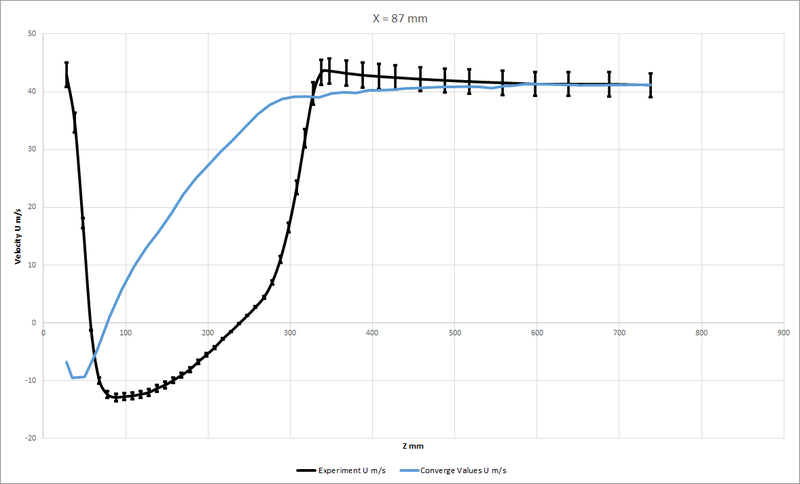
We have some experimental data from “S. Becker, H. Lienhart, C. Stoots, ERCOFTAC workshop 9.4(2000): LDA-Measurement”. They collected the velocity along x-direction at different locations along the X and Z axes using probes And plotted some graphs with that data. This data can be found here. We are going to do the same in a virtual system.

Using the plot over line option in paraview we can extract the velocity in the X direction at different locations along the X and Z axes. The plot over line command plots the Z location Vs velocity along X for different X locations. We use the export scene option to export this plot data into an excel sheet.

We take both the experimental data and the simulated data and plot them in a single graph we get the following graphs for different locations.

@ x = -13 mm

@ x = -263 mm

@ x = 37 mm

@ x = 87 mm

@ x = -113 mm

@ x = -63 mm

@ x = 187 mm

@ x = 137 mm

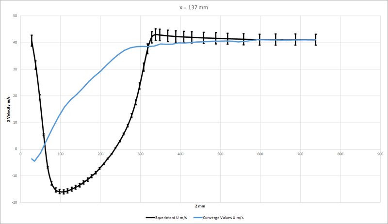
The spikes in the above graphs indicate an error percentage of 5%. The above plots are for different locations along X. We can to normalise the above data using octave and put them in a single graph it would look like this

Now that we have got all our data we calculate the lift and drag coefficients.

we know that lift force F_l = 1/2C_l*rho*A*V^2

Where C_lis the Lift coefficient and A is the wing Area in terms of aeronautics. This is an area upon which the lift is produced by Bernoulli’s principle. This is the product of the wingspan and chord length. In our terms, it is (1044*398) mm^2.

Drag force F_d = 1/2*C_d*rho*A*V^2

Where C_d is the drag coefficient and A is the frontal area. This can be extracted from paraview

It is nothing but (389*288)mm^2

we can also extract the drag and lift forces using the post processing tools. Once the drag and lift force values are extracted we can use octave to calculate the mean of these values.

we plug in these values in the above equations to find out the drag and lift coefficients.

The results are as follows.

CONCLUSION:

From the graphs, we can see that the probes at the negative location are matching well with the experimental data compared to the probes on the positive side.

On the positive side, we can see that the error percentage in the graphs is greater than 5%. This could be because of various reasons but the overall trend of the curve remains the same. Grid size could be a possible factor.

The error on the positive side is greater because of the Drag produced on the rear side of the body. The rear side is positive from origin.

To capture this wake region correctly a smaller grid size and greater computational power are required.

The air after exiting the cylindrical pillars forms vortices. These vortices can be observed from the top view. It is also observed that the lift obtained is negative which means that it is downward force. This force helps racing cars to stay on the ground. But for a low-efficiency vehicle such as a truck, this force is not desirable. Hence the shape of the truck/trailer will be optimized to reduce the negative lift.

From the Velocity contour, it is observed that after passing through the geometry there is a region where recirculation happens this region is called as wake region. Due to this low pressure, the air at the front tries to come back which causes the Pressure drag.

On reducing the grid size the Cd and Cl values increases by some extent implying the solution is grid dependent. But the minor increase indicates that by the next lower size the solution may stabilise and become grid dependent.

REFERENCES:

The Ahmed Body

The viscosity of Air, Dynamic and Kinematic

Experiments and numerical simulations on the aerodynamics of the Ahmed body

presentation-Milano-MoellerSuzzi The viscosity of Air, Dynamic and Kinematic