
1D Supersonic Nozzle flow simulation using MacCormac Method
AIM:
Aim of this project is to model the Isentropic flow through a quasi 1D subsonic-supersonic nozzle using mathematical equations and solve the equations to simulate a flow.
OBJECTIVES :
The objectives of this project are
To solve the equations that govern the flow through a supersonic nozzle for both conservative and non conservative forms.
To find the differences between them by comparing their solutions.
Steady-state distribution of primitive variables inside the nozzle. Time-wise variation of the primitive variables.
Variation of Mass flow rate distribution inside the nozzle at different time steps during the time-marching process.
Comparison of Normalized mass flow rate distributions of both forms. Perform a grid independence test on the solution.
THEORY:
we assume that the flow is quasi 1D i.e the flow is only along the x-axis and any change in flow along y-axis is negligible. (Taken from CFD Basics by John Anderson)

To simulate the flow we need to do the following steps
1.Mesh Generation/Meshing is the process of divinding a continuous geometry into discrete geometric cells. Each cell is seperated by a node. These nodes form The Grid.
2.Discretisation is the process of converting the above PDEs into algebraic equations
3.Solving the discretised PDEs. Based on the type of PDEs different methods are chosen. The type of PDE in our case is hyperbolic so we are using the Mac Cormac method
MacCormac Method is an explicit finite difference technique which is second order accurate for both space and time. It is easy to work with and the solutions obtained are stable. The procedure is as follows
1.Predictor step: Here we use the numerical method to calculate the required derivatives using the forward differencing scheme.
2.Solution update: We add the change obtained in the above step to the original variable.
3.Primitive Variables: (Only for conservative form )For the conservative form we calculate the primitive variables from the solution vectors, flux vectors and source terms.
4.Corrector Step: We use the numerical method to calculate the same derivatives we calculated in the first step again using the backward differencing scheme.
5.Calculating the average: We take the average of derivatives we obtained in step 1 and step 4.
6.Final solution update: we add the final change we calculated in step 5 to the original variable. This would be the final answer.
Here we will be solving the equations in conservative and non conservative forms which will be one of the key objectives. Conservative and Non conservative forms are basically the same equations but the method considered to solve the deriavatives will differ.
For eg,
consider a derivative
$$ \frac{\partial \rho u}{\partial x} $$
the conservative form would solve it like
$$ \frac{\rho u_i - \rho u_{i-1}}{\Delta x} $$
where as the non conservative form would solve it like
$$ \rho\frac{\partial u}{\partial x} + u\frac{\partial \rho}{\partial x} $$
To understand the impact this will have on the solution we will simulate the supersonic flow we solve the flow equations of both the forms i.e.,
Non Conservative form:-
There are three main equations for
Continuity : $$\frac{\partial \rho}{\partial t} + v \cdot \frac{\partial (\rho A)}{\partial x} = - \rho A \frac{\partial v}{\partial x}$$
Momentum : $$\rho \frac{\partial v}{\partial t} + \rho v \frac{\partial v}{\partial x} = -\frac{\partial p}{\partial x}$$
Energy : $$\rho \frac{\partial e}{\partial t} + \rho v \frac{\partial e}{\partial x} = - p \frac{\partial v}{\partial x} - p v \frac{\partial (\ln A)}{\partial x}$$
We non dimensionalise the given equations to ease our matlab programming. So new terms are
$$x’ = \frac{x}{L}, v’ = \frac{v}{a_0}, T’ = \frac{T}{\frac{L}{a_0}}, A’ = \frac{A}{A^0}$$
Non dimensionalised equations are
Continuity : $$\frac{\partial \rho’}{\partial t’} = - \rho’ \frac{\partial v’}{\partial x’} - \rho’ v’ \frac{\partial (\ln A’)}{\partial x’} - v’ \frac{\partial \rho’}{\partial x’}$$
Momentum :$$\frac{\partial v’}{\partial t’} = - v’ \frac{\partial v’}{\partial x’} - \frac{1}{\gamma} \left( \frac{\partial T’}{\partial x’} + \frac{T’}{\rho’} \frac{\partial \rho’}{\partial x’} \right)$$
Energy : $$\frac{\partial T’}{\partial t’} = - v \frac{\partial T’}{\partial x’} - (\gamma - 1) T’ \left( \frac{\partial v’}{\partial x’} + v’ \frac{\partial (\ln A’)}{\partial x’} \right)$$
Conservative form:-
The non dimensionalised equations are
Continuity : $$\frac{\partial (\rho’ A’)}{\partial t} + \frac{\partial (\rho’ A’ v’)}{\partial x’} = 0$$
Momentum : $$\frac{\partial (\rho’ A’ v’)}{\partial t’} + \frac{\partial \left( \rho’ A’ v’^2 + \frac{1}{\gamma} p’ A’ \right)}{\partial x’} = - \frac{1}{\gamma} p’ \frac{\partial A’}{\partial x’}$$
Energy : $$\frac{\partial \left( \rho’ \left( \frac{T’}{\gamma - 1} + \frac{\gamma}{2} v’^2 \right) A’ \right)}{\partial t’} + \frac{\partial \left( \rho’ \left( \frac{T’}{\gamma - 1} + \frac{\gamma}{2} v’^2 \right) A’ + p’ A’ v’ \right)}{\partial x’} = 0$$
The above equations cant be programmed into MATLAB, So we break the above equation into Flux terms and solution vectors
Flux Term:-
$$F_1 = \rho’ A’ v’$$
$$F_2 = \rho’ A’ v’^2 + \frac{1}{\gamma} p’ A’$$
$$F_3 = \rho’ \left( \frac{T’}{\gamma - 1} + \frac{\gamma}{2} v’^2 \right) v’ A’ + p’ A’ v’$$
Solution Vectors:-
$$U_1 = \rho ’ A ’ $$
$$U_2 = \rho ’ A ’ v ’ $$
$$U_3 = \rho \left( \frac{T}{\gamma - 1} + \frac{\gamma}{2} v’^2 \right) A’$$
Source Term:-
$$J_2 = \frac{1}{\gamma} p \frac{\partial A’}{\partial x’}$$
These equations are now used to solve a problem by providing some inputs, intial conditions and boundary conditions. These are different for conservative and non conservative. A common quantity that doesnt change with the conservative and non conservative form is the profile of the nozzle. This is defined using the area of the nozzle. For this project the area is taken in the form of a parabolic curve which is denoted by
$$ A = 1 + 2.2 (x − 1.5 ) ^ {2}$$
The throat of the nozzle is at x = 1.5 the convergent section occurs at x < 1.5 and the divergent section occurs at x > 1.5. The curve would look like this (Image courtesy CFD Basics by John D Anderson)

We try to simulate the program for a time of 1400 timesteps and the length of the nozzle is taken as 3 units which is divided into 31 nodes. The timestep provided is such that it satisfies the CFL criteria. If the timestep provided doesnt satisfy the CFL criteria the solution will blow up.
For conservative form the inputs are
Initial conditions:
For $$0 ⩽ x ⩽ 0.5 ; \rho ’ = 1.0 , T ’ = 1.0$$
For $$0.5 ⩽ x ⩽ 1.5 ; \rho ’ = 1.0 − 0.366(x ’ − 0.5) ; T ’ = 1.0 − 0.167(x ’ − 0.5)$$
For $$ 1.5 ⩽ x ⩽ 3.5 ; \rho ’ = 0.634 − 0.3879 (x ’ − 1.5 ) ; T ’ = 0.833 − 0.3507 (x ’ − 1.5)$$
$$v’ = U_2 = \frac{0.59}{\rho’ A’} ; p’ = \rho’ T’ ; M = \frac{v’}{\sqrt{T’}}$$
Boundary conditions:
Inlet:
$$U_1 (1) = \rho’ (1 ) ∗ a’ (1) $$;
$$U_2 (1) = 2 ∗ U_2(2) - U_2(3)$$
$$U_3 (1 ) = U_1 (1 ) ∗ ({T (1)} / {(\gamma − 1)} + {\gamma} / {2} ∗ v (1) ^ {2}) ;$$
$$V_1(1 ) = {U_2 (1 )} / {U_1 (1 )} ;$$
Outlet:
$$U_1 (n ) = 2 ∗ U_1 (n − 1 ) − U_1 (n − 2 ) ;$$
$$U_2 (n ) = 2 ∗ U_2 (n − 1 ) − U_2 (n − 2 ) ;$$
$$ U_3 (n ) = 2 ∗ U_3 (n-1 ) − U_3 (n-2 ) ;$$
If everything is in place the code for the conservative form should look like this
%%%%%%%%%%%%%%%%%%%%%%%%%%%%%%%%%%%%%%%%%%%%%%%%%%%%%%%%%%%%%%%%%%%%%%%%%
%%%%%%%%%%%%%%%%%%%%% CONSERVATIVE FORM %%%%%%%%%%%%%%%%%%%%%%%%%%%%%%%%%
%%%%%%%%%%%%%%%%%%%%%%%%%%%%%%%%%%%%%%%%%%%%%%%%%%%%%%%%%%%%%%%%%%%%%%%%%

function  [x, a, mfr, v_c, v_throat, rho_c, rho_throat, T_c, T_throat, p_c, p_throat, M_c , M_throat] = conserfunc(n,x,dx,gamma,nt)

%The programming from here on is referenced from CFD Basics by John D Anderson, Jr.

rho_c = ones(1,n);
T_c = 300*ones(1,n);

%Intial Conditions
for i =1:n
   if (x(i) >= 0 && x(i) <= 0.5)
       rho_c(i) = 1;
       T_c(i) = 1;

   elseif (x(i) > 0.5 && x(i) < 1.5)
       rho_c(i) = 1 - 0.366*(x(i) - 0.5);
       T_c(i) = 1 - 0.167*(x(i)-0.5);

   elseif (x(i) >= 1.5 && x(i) <= 3.5)
       rho_c(i) = 0.634 - 0.3879*(x(i) - 1.5);
       T_c(i) = 0.833 - 0.3507*(x(i) - 1.5);

   end
end

a = 1 + 2.2*(x-1.5).^2;%(Area) same as the non conservative form since
%area profile is same as a parabolic nozzle for both the forms

%to find out the throat section
N = find(a==1);

%Initial velocity is taken according to the initial conditions specified in the book
v_c = 0.59./(rho_c.*a);

%The non dimensional conservative form of equations are expressed in terms
%of solution vectors and flux terms

%SOLUTION VECTORS
U1 = rho_c.*a;

U2 = rho_c.*a.*v_c;

U3 = rho_c.*a.*((T_c/(gamma -1))+(gamma*0.5*(v_c.^2)));

%FLUX VECTORS
F1 = U2;

F2 = ((U2.^2)./U1)+((gamma-1)/gamma)*(U3 - (gamma/2)*(U2.^2)./U1);

F3 = ((gamma*U2.*U3)./(U1)) - ((gamma*(gamma-1))/2)*((U2.^3)./(U1.^2));


%outer time loop
for k = 1:nt
    %initiation of Uold values
    U1_old = U1;

    U2_old = U2;

    U3_old = U3;

    %time step number is dependent on courant number
    %we gave the inputs such that CFL criteria is satisfied C*dx/dt <= 0.5 ;
    dt = min(0.5*dx./(v_c+sqrt(T_c)));

    %predictor step
    for j = 2:n-1

        F1(j) = U2(j);

        F2(j) = ((U2(j)^2)/U1(j))+((gamma-1)/gamma)*(U3(j) - (gamma/2)*(U2(j)^2/U1(j)));

        F3(j) = ((gamma*U2(j)*U3(j))/(U1(j))) - (gamma*(gamma-1)/2)*(U2(j)^3/U1(j)^2);

        dF1_dx(j) = (F1(j+1)-F1(j))/dx;

        dF2_dx(j) = (F2(j+1)-F2(j))/dx;

        dF3_dx(j) = (F3(j+1)-F3(j))/dx;

        dadx(j) = (a(j+1)-a(j))/dx ;

        J2(j) = (1/gamma)*rho_c(j)*T_c(j)*dadx(j);

        %solving for continuity equation
        dU1_dt_p(j) = -dF1_dx(j);

        %solving for momentum equation
        dU2_dt_p(j) = -dF2_dx(j)+J2(j);

        %solving for energy equation
        dU3_dt_p(j) = -dF3_dx(j);

        %solution update
        U1(j) = U1(j) + dU1_dt_p(j)*dt;%updating velocity

        U2(j) = U2(j) + dU2_dt_p(j)*dt;%updating Temperature

        U3(j) = U3(j) + dU3_dt_p(j)*dt;%Updating density

    end

    %Decoding Primitive variables from U1, U2 and U3
    rho_c = U1./a;

    v_c = U2./U1;

    T_c = (gamma - 1)*((U3./U1)-(gamma*0.5.*(v_c.^2)));

    %calculating the predicted values of flux terms
    F1 = U2;

    F2 = ((U2.^2)./U1)+((gamma-1)/gamma)*(U3 - ((gamma/2)*((U2.^2)./U1)));

    F3 = ((gamma*U2.*U3)./(U1)) - ((gamma*(gamma-1)/2)*((U2.^3)./(U1.^2)));

    %corrector step
    for j = 2:n-1

        dF1_dx(j) = (F1(j)-F1(j-1))/dx;

        dF2_dx(j) = (F2(j)-F2(j-1))/dx;

        dF3_dx(j) = (F3(j)-F3(j-1))/dx;

        dadx(j) = (a(j)-a(j-1))/dx ;

        J2(j) = (1/gamma)*rho_c(j)*T_c(j)*dadx(j);

        %solving for continuity equation
        dU1_dt_c(j) = -dF1_dx(j) ;

        %solving for momentum equation
        dU2_dt_c(j) = -dF2_dx(j)+J2(j);

        %solving for energy equation
        dU3_dt_c(j) = -dF3_dx(j);

    end

    %avg of predictor and corrector

    dU1_dt = 0.5*(dU1_dt_p + dU1_dt_c);

    dU2_dt = 0.5*(dU2_dt_p + dU2_dt_c);

    dU3_dt = 0.5*(dU3_dt_p + dU3_dt_c);

    %final solution update

    for i = 2:n-1

        U1(i) = U1_old(i) + (dU1_dt(i)*dt);

        U2(i) = U2_old(i) + (dU2_dt(i)*dt);

        U3(i) = U3_old(i) + (dU3_dt(i)*dt)  ;
    end

    %Applying the boundary conditions
    %inlet
    U1(1) = rho_c(1)*a(1);

    U2(1) = 2*U2(2)-U2(3);

    U3(1) = U1(1)*((T_c(1)/(gamma -1))+(gamma*0.5*(v_c(1)^2)));

    v_c(1) = U2(1)/U1(1);

    %outlet
    U1(n) = 2*U1(n-1)-U1(n-2);

    U2(n) = 2*U2(n-1)-U2(n-2);

    U3(n) = 2*U3(n-1)-U3(n-2);

    %primitive variables

    rho_c = U1./a;

    v_c = U2./U1;

    T_c = (gamma - 1)*((U3./U1)-(gamma*0.5.*(v_c.^2)));

    %calculating the properties

    p_c = rho_c.*T_c;% Pressure

    M_c = v_c./sqrt(T_c) ;% Mach number

    mfr = rho_c.*a.*v_c;% Mass Flow Rate

    %Paraneter values at the throat section

    rho_throat(k) = rho_c(N); %density

    v_throat(k) = v_c(N); %velocity

    T_throat(k) = T_c(N); %Temperature

    M_throat(k) = M_c(N); %Machnumver

    p_throat(k) = p_c(N); %Pressure

    figure(1)
    if k == 1
        plot(x,mfr)
        hold on
    elseif k == 50
        plot(x,mfr)
        hold on
    elseif k == 100
        plot(x,mfr)
        hold on
    elseif k == 200
        plot(x,mfr)
        hold on
    elseif k == 600
        plot(x,mfr)
        hold on
    elseif k == 800
        plot(x,mfr)
        hold on
    elseif k == 1000
        plot(x,mfr)
        hold on
    xlabel('Non dimensionalised "X"')
    ylabel('Mass Flow rate')
    legend('1st timestep','50th timestep','100th timestep','200th timestep','600th timestep','800th timestep','1000th timestep')
    grid on
    title('Conservation analysis Mass flow rate at different timesteps')
    end
end

end
For Non conservative form the inputs are
Initial conditions:
$$\rho = 1 - 0.3146∗ x$$
$$T = 1- 0.2314∗ x$$
$$v = (0.1 + 1.09∗ x)∗ sqrt T$$
Boundary conditions:
Inlet:
$$v (1 ) = 2 ∗ v (2 ) − v (3 ) ;$$
Outlet:
$$\rho (n ) = 2 ∗ \rho (n-1 ) − \rho (n-2 ) ;$$
$$T (n ) = 2 ∗ T (n-1 ) − T (n-2 ) ;$$
$$v (n ) = 2 ∗ v (n-1 ) − v (n-2 ) ;$$
If everything is in place the code for the conservative form should look like this
%%%%%%%%%%%%%%%%%%%%%%%%%%%%%%%%%%%%%%%%%%%%%%%%%%%%%%%%%%%%%%%%%%%%%%%%%
%%%%%%%%%%%%%%%%% NON CONSERVATIVE FORM %%%%%%%%%%%%%%%%%%%%%%%%%%%%%%%%%
%%%%%%%%%%%%%%%%%%%%%%%%%%%%%%%%%%%%%%%%%%%%%%%%%%%%%%%%%%%%%%%%%%%%%%%%%

function [x, a, mfr, v_nc, v_throat, rho_nc, rho_throat, T_nc, T_throat, p_nc, p_throat, M_nc, M_throat] = nonconserfunc(n,x,dx,gamma,nt)

%Providing inputs
%Since all the inputs are converted into non dimensionalised form
%They are expressed in the form of x

rho_nc = 1 - 0.3146*x;%(density)

T_nc = 1-0.2314*x;%(Temperature)

v_nc = (0.1 + 1.09*x).*T_nc.^0.5;%(Velocity)

a = 1 + 2.2*(x-1.5).^2;%(Area)


%time step number is dependent on courant number
%we gave the inputs such that CFL criteria is satisfied C*dx/dt <= 0.5 ;
dt = 0.01;%min(0.5*dx./(v_nc+sqrt(T_nc)));

%To get better results we calculate the values at the throat section
%seperately
N = find(a==1);

%outer time step loop
for k = 1:nt

    %we save the old values here
    rho_old = rho_nc;

    v_old = v_nc;

    T_old = T_nc;

    %predictor step
    for j = 2:n-1

        dvdx = (v_nc(j+1)-v_nc(j))/dx;

        drhodx =(rho_nc(j+1)-rho_nc(j))/dx;

        dTdx = (T_nc(j+1)-T_nc(j))/dx;

        dlog_adx = (log(a(j+1))-log(a(j)))/dx ;

        %solving for continuity equation
        drho_dt_p(j) = -rho_nc(j)*(dvdx) -rho_nc(j)*v_nc(j)*dlog_adx - v_nc(j)*drhodx ;

        %solving for momentum equation
        dv_dt_p(j) = -v_nc(j)*(dvdx)- (1/gamma)*(dTdx+((T_nc(j)/rho_nc(j))*(drhodx)));

        %solving for energy equation
        dT_dt_p(j) = -v_nc(j)*dTdx- (gamma -1)*(T_nc(j))*(dvdx + v_nc(j)*(dlog_adx));

        %solution update
        v_nc(j) = v_old(j) + dv_dt_p(j)*dt;%updating velocity

        T_nc(j) = T_old(j) + dT_dt_p(j)*dt;%updating Temperature

        rho_nc(j) = rho_old(j) + drho_dt_p(j)*dt;%Updating density
    end

    %corrector step
    for j = 2:n-1

        dvdx = (v_nc(j)-v_nc(j-1))/dx;

        drhodx =(rho_nc(j)-rho_nc(j-1))/dx;

        dTdx = (T_nc(j)-T_nc(j-1))/dx;

        dlog_adx = (log(a(j))-log(a(j-1)))/dx ;

        %solving for continuity equation
        drho_dt_c(j) = -rho_nc(j)*(dvdx) -rho_nc(j)*v_nc(j)*dlog_adx - v_nc(j)*drhodx ;

        %solving for momentum equation
        dv_dt_c(j) = -v_nc(j)*(dvdx)- (1/gamma)*(dTdx+((T_nc(j)/rho_nc(j))*(drhodx)));

        %solving for energy equation
        dT_dt_c(j) = -v_nc(j)*(dTdx)- (gamma -1)*(T_nc(j))*(dvdx + v_nc(j)*(dlog_adx));

    end

    %avg of predictor and corrector

    dv_dt = 0.5*(dv_dt_p + dv_dt_c);

    drho_dt = 0.5*(drho_dt_p + drho_dt_c);

    dT_dt = 0.5*(dT_dt_p + dT_dt_c);

    %final solution update

    for i = 2:n-1

        v_nc(i) = v_old(i) + dv_dt(i)*dt;

        rho_nc(i) = rho_old(i) + drho_dt(i)*dt;

        T_nc(i) = T_old(i) + dT_dt(i)*dt;

    end

    %Apply the boundary conditions
    %inlet
    v_nc(1) = 2*v_nc(2) - v_nc(3);

    %outlet
    v_nc(n) = 2*v_nc(n-1) - v_nc(n-2);

    rho_nc(n) = 2*rho_nc(n-1) - rho_nc(n-2);

    T_nc(n) = 2*T_nc(n-1) - T_nc(n-2);

    %calculating the properties

    p_nc = rho_nc.*T_nc; % Pressure

    M_nc = v_nc./(T_nc.^0.5) ; % Mach Number

    mfr = rho_nc.*a.*v_nc; % Mass Flow Rate

    %Parameter value at the throat section

    rho_throat(k) = rho_nc(N); %Density

    v_throat(k) = v_nc(N); %Velocity

    T_throat(k) = T_nc(N); %Temperature

    M_throat(k) = M_nc(N); %Mach number

    p_throat(k) = p_nc(N); %Pressure

    figure(2)
    if k == 1
        plot(x,mfr)
        hold on
    elseif k == 50
        plot(x,mfr)
        hold on
    elseif k == 100
        plot(x,mfr)
        hold on
    elseif k == 200
        plot(x,mfr)
        hold on
    elseif k == 600
        plot(x,mfr)
        hold on
    elseif k == 800
        plot(x,mfr)
        hold on
    elseif k == 1000
        plot(x,mfr)
        hold on
    xlabel('Non dimensionalised "X"')
    ylabel('Mass Flow rate')
    legend('1st timestep','50th timestep','100th timestep','200th timestep','600th timestep','800th timestep','1000th timestep')
    grid on
    title('Non Conservation analysis Mass flow rate at different timesteps')
    end

end

end
Along with everything mentioned above we also calculate the mach number over the entire non dimensional distance.Now we call the two functions into a main program which will provide the data we need. If everything is in place the main program should look like this
clear
close all
clc

%%%%%%%%%%%%%%%%%%%%%%%%%%%%%%%%%%%%%%%%%%%%%%%%%%%%%%%%%%%%%%%%%%%%%%%%%%%%%%%%%%%%%
%%% SOLVING THE 1D SUPERSONIC NOZZLE FLOW EQUATIONS USING THE MACCORMAC METHOD %%%%%%
%%%%%%%%%%%%%%%%%%%%%%%%%%%%%%%%%%%%%%%%%%%%%%%%%%%%%%%%%%%%%%%%%%%%%%%%%%%%%%%%%%%%%

% inputs
n = 31;
x = linspace(0,3,n);
dx = x(2)-x(1);
gamma = 1.4;

%defining time steps
nt = 1400;
wt = linspace(1,nt,nt);

%calling the conservative form function
[x, a, mfr_c, v_c, v_cthroat, rho_c, rho_cthroat, T_c, T_cthroat, p_c, p_cthroat, M_c , M_cthroat] = conserfunc(n,x,dx,gamma,nt);
%calling the non conservative form function
[x, a, mfr_nc, v_nc, v_ncthroat, rho_nc, rho_ncthroat, T_nc, T_ncthroat, p_nc, p_ncthroat, M_nc , M_ncthroat] = nonconserfunc(n,x,dx,gamma,nt);

%from the book
mfr_a = 0.579*ones(1,n);

%for the grid dependecy test
%conservative terms
pcmean = mean(p_cthroat);
rhocmean = mean(rho_cthroat);
Tcmean = mean(T_cthroat);
Mc_mean = mean(M_cthroat);

%Nonconservative terms
pncmean = mean(p_ncthroat);
rhoncmean = mean(rho_ncthroat);
Tncmean = mean(T_ncthroat);
Mnc_mean = mean(M_ncthroat);

%plotting
% Parameters change with X axis
figure(3)

subplot(4,1,1)
grid on
plot(x,rho_nc,'b','linewidth',4)
hold on
plot(x,rho_c,'color','r','linewidth',2)
ylabel('Density')
legend('Non conservative','conservative')

subplot(4,1,2)
grid on
plot(x,T_nc,'b','linewidth',4)
hold on
plot(x,T_c,'color','r','linewidth',2)
ylabel('Temperature')
legend('Non conservative','conservative')

subplot(4,1,3)
grid on
plot(x,p_nc,'b','linewidth',4)
hold on
plot(x,p_c,'color','r','linewidth',2)
ylabel('Pressure')
legend('Non conservative','conservative')

subplot(4,1,4)
grid on
plot(x,M_nc,'b','linewidth',4)
hold on
plot(x,M_c,'color','r','linewidth',2)
ylabel('Mach number')
xlabel('X')
legend('Non conservative','conservative')

%Throat parameters
figure(4)
subplot(4,1,1)
grid on
plot(wt,rho_ncthroat)
hold on
plot(wt,rho_cthroat)
ylabel('Density')
legend('Non conservative','conservative')
title('Variation of flow properties with timestep at throat')

subplot(4,1,2)
grid on
plot(wt,T_ncthroat)
hold on
plot(wt,T_cthroat)
ylabel('Temperature')
legend('Non conservative','conservative')

subplot(4,1,3)
grid on
plot(wt,p_ncthroat)
hold on
plot(wt,p_cthroat)
ylabel('Pressure')
legend('Non conservative','conservative')

subplot(4,1,4)
grid on
plot(wt,M_ncthroat)
hold on
plot(wt,M_cthroat)
ylabel('Mach number')
xlabel('Time Step')
legend('Non conservative','conservative')

%Mass flow rate comparision
figure(5)
grid on
plot(x,mfr_nc)
hold on
plot(x,mfr_c)
plot(x,mfr_a)
xlabel('Non-Dimensionalised distance')
ylabel('Mass Flow Rate')
legend('Non conservative','conservative','Exact analytical solution')
title('Comparision for Conservative and Non-conservative Mass Flow Rate')

%For ease of extraction of data a table has been created
figure(6)
set(gcf,'position',[20 20 700 120])
col = {'Grid points','Pressure','Density','Temperature','Machnumber'};
row = {'Conservative','Non Conservative'};
dat = {n,pcmean,rhocmean,Tcmean,Mc_mean;n,pncmean,rhoncmean,Tncmean,Mnc_mean};
uitable('columnname',col,'rowname',row,'Data',dat,'columnwidth',{100},'position',[15 15 680 100]);
we get the following graphs once we run the program.
RESULTS

OBSERVATION
In the above figure we can see how the variables change over the non dimensionalied distance. We can observe that at the throat section i.e., at x’ = 1.5 the mach number seems to increase indicating the flow is changing from subsonic to supersonic over the nozzle. Also all the remaining variables change as they would over a nozzle in a practical situation. The pressure is compensated for an increase in velocity.


OBSERVATION
From the above graphs we can observe that the mass flowrate tends to stabilise from 600th timestep and at 1000th timestep it is completely stable. Also we can observe that the Non conservative mass flow rate has more deviation than the conservative timestep this can be correlated with how the differentials are treated.

OBSERVATION
From the above graph it is observed that the mass flow rate with the conservative form is closer to exact solution and has less deviations compared to non conservative form.

OBSERVATION
From the above graph we can say that both conservative and non conservative forms have deviations in the beginning of the time marching. But the conservative form had relatively less deviations compared to non conservative flow. Over the time both have converged into a single exact solution.
GRID INDEPENDENCE TEST:
This is an important test we conduct to know if the solution relies on the grid size or not. If the solution relies on the grid size then the solution cannot be trusted.
we take the mean of values at the throat section i.e where the area is equal to 1
16th node for 31 grid points and 31st node for 61 grid points.
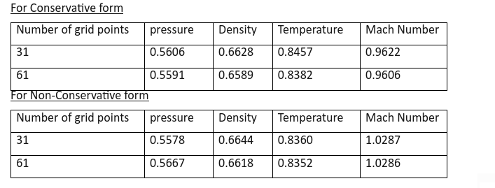
For our tolerance level we can say that the solution is grid independent
CONCLUSION:
We have mathematically modelled a isentropic supersonic flow using the Mac cormac FDM method. We have used both conservative and non conservative forms. From the above data we can conclude the non conservative form has more deviations with the initial guesses and more offset from the analytical solution compared to the conservative form. The idea is that with the compressible flows conservative form works the best while for incompressible flows non conservative form will give a better trade off for solution accuracy and computational resources.